6. 特征工程(FetureEngineering)
特征是数据中抽取出来的对结果预测有用的信息,可以是文本或者数据。
特征工程是使用专业背景知识和技巧处理数据,使得特征能在机器学习算法上发挥更好的作用的过程。过程包含了数据清洗, 特征提取, 特征构建、特征选择等模块。
特征工程的目的是筛选出更好的特征,获取更好的训练数据。因为好的特征具有更强的灵活性,可以用简单的模型做训练,更可以得到优秀的结果。
6.1. 分类特征
一种常见的数据是分类数据,比如鸢尾花中最终的结果,我们用数字表示三种鸢尾花中的一种,比如这样:
rst = {"setosa":1, "versicolor":2, "virginica": 3}
但这种可能会造成错觉,因为数字经常会暗含一些关系在其中,比如如果不加说明很容易让人理解成:
sentosa < versicolor < virginica
或者
virginica = setosa + versicolor
但是我们知道这种关系肯定是不对的,我们人类可能误解其中的关系,计算机同样也可能。
面对这样的情况,我们经常采用独热编码(OneHotCoding)进行处理,即增加额外的列,让0和1出现在对应的列表示每个分类的值有或者无。
SKlearn中的DictVectorizer可以把分类编码转换成独热编码。
from sklearn.feature_extraction import DictVectorizer

#准备数据
stu = [
    {'age': 19, "height":187, "name":"刘大拿", "room":"Class01"},
    {'age': 29, "height":177, "name":"刘二拿", "room":"Class02"},
    {'age': 59, "height":181, "name":"刘三拿", "room":"Class03"},
]

vec = DictVectorizer(sparse=False, dtype=int)
c = vec.fit_transform(stu)

print("特征名称为: {}\n".format(vec.get_feature_names()))
print("编码后数据为:\n {} \n".format(c))
print(c.shape)
特征名称为: ['age', 'height', 'name=刘三拿', 'name=刘二拿', 'name=刘大拿', 'room=Class01', 'room=Class02', 'room=Class03']

编码后数据为:
 [[ 19 187   0   0   1   1   0   0]
 [ 29 177   0   1   0   0   1   0]
 [ 59 181   1   0   0   0   0   1]]

(3, 8)
这种做法会很大程度增加数据维度,以至于带来其他的问题。
独热编码因为编码原理,会有很多0出现,这种矩阵使用稀疏矩阵来处理比较好。
# 参数sparse=True表明使用稀疏矩阵存储编码
vec = DictVectorizer(sparse=True, dtype=int)
c = vec.fit_transform(stu)

print("采用稀疏矩阵存储后的数据:\n {}\n".format(c))
采用稀疏矩阵存储后的数据:
   (0, 0)	19
  (0, 1)	187
  (0, 4)	1
  (0, 5)	1
  (1, 0)	29
  (1, 1)	177
  (1, 3)	1
  (1, 6)	1
  (2, 0)	59
  (2, 1)	181
  (2, 2)	1
  (2, 7)	1
6.2. 文本特征
文本特征抽取常见的比如单词统计,词频统计等。
下面举例对文本单词数量进行统计。
#准备数据
sample  = ['beijing tuling xueyuan is the zui niubility',
'Because the people who are crazy enough to think that they can change the world, are the ones who do',
'gone with the wind']

from sklearn.feature_extraction.text import CountVectorizer

vec = CountVectorizer()
X = vec.fit_transform(sample)
print(type(X))
print(X)
print("FeaturesNames: \n {}".format(vec.get_feature_names()))
<class 'scipy.sparse.csr.csr_matrix'>
  (0, 2)	1
  (0, 18)	1
  (0, 23)	1
  (0, 9)	1
  (0, 14)	1
  (0, 24)	1
  (0, 10)	1
  (1, 14)	3
  (1, 1)	1
  (1, 12)	1
  (1, 19)	2
  (1, 0)	2
  (1, 5)	1
  (1, 7)	1
  (1, 17)	1
  (1, 16)	1
  (1, 13)	1
  (1, 15)	1
  (1, 3)	1
  (1, 4)	1
  (1, 22)	1
  (1, 11)	1
  (1, 6)	1
  (2, 14)	1
  (2, 8)	1
  (2, 21)	1
  (2, 20)	1
FeaturesNames:
 ['are', 'because', 'beijing', 'can', 'change', 'crazy', 'do', 'enough', 'gone', 'is', 'niubility', 'ones', 'people', 'that', 'the', 'they', 'think', 'to', 'tuling', 'who', 'wind', 'with', 'world', 'xueyuan', 'zui']
以上结果是一个稀疏矩阵,我们可以把稀疏矩阵还原成DataFrame格式。
import pandas as pd

#稀疏矩阵还原成DataFrame格式
df = pd.DataFrame(X.toarray(), columns=vec.get_feature_names())

print("表格形式数据为:\n", df)
表格形式数据为:
    are  because  beijing  can  change  crazy  do  enough  gone  is ...   they  \
0    0        0        1    0       0      0   0       0     0   1 ...      0
1    2        1        0    1       1      1   1       1     0   0 ...      1
2    0        0        0    0       0      0   0       0     1   0 ...      0

   think  to  tuling  who  wind  with  world  xueyuan  zui
0      0   0       1    0     0     0      0        1    1
1      1   1       0    2     0     0      1        0    0
2      0   0       0    0     1     1      0        0    0

[3 rows x 25 columns]
当然上面是最粗略的统计,在统计文本的过程中,经常使用的是TF-IDF(Term FrequencyInverseDocumentFrequency),在文本处理的章节我们会单独讲述。
6.3. 衍生特征
有时候我们需要用到当前数据没有的特征,这类特征可以从现有数据进行处理后的出来,此类特征叫衍生特征,属于无中生有系列。
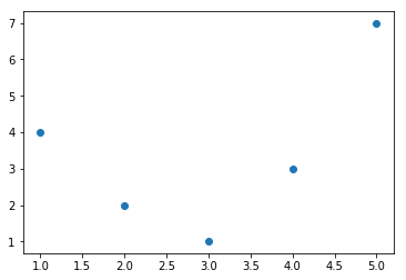
基函数回归经常要用到衍生特征,参看下面案例。
%matplotlib inline

import numpy as np
import matplotlib.pyplot as plt

x = np.array([1,2,3,4,5])
y = np.array([4,2,1,3,7])

plt.scatter(x,y)
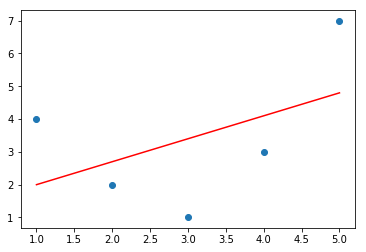
我们对上面图形进行线性回归拟合,最终会得到一条直线,但很显然这并不能满足我们的需求。
from sklearn.linear_model import LinearRegression

X = x[:, np.newaxis]

model = LinearRegression().fit(X, y)

yfit = model.predict(X)
plt.scatter(x, y)
plt.plot(x, yfit, c="red")
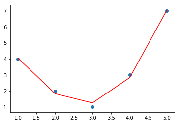
根据观察,对于上面数据拟合如果能采用更复杂的模型, 比如二次多项式或者三次多项式应该会获得比较满意的结果,我们采用多项式回归模型。
from sklearn.preprocessing import PolynomialFeatures

poly = PolynomialFeatures(degree=3, include_bias=False)

#对数据进行衍生特征处理,线有数据不能满足三次多项式模型的需求
X2 = poly.fit_transform(X)
print(X2.shape)

model = LinearRegression().fit(X2, y)
yfit = model.predict(X2)

plt.scatter(x, y)
plt.plot(x, yfit, c='red')
6.4. 缺失值填充
对缺失值进行填充,我们前面数据科学入门中有过讲述,但在sklearn中我们可以直接使用工具来完成,更直接迅速。
from numpy import nan

X = np.array([[nan, 3, 2],
            [3, 2, 12],
            [9, nan, 21],
            [3,4,nan],
            [1,2,5]])


# Imputer帮助我们完成填充
from sklearn.impute import SimpleImputer


#填充策略使用平均值
imp = SimpleImputer(strategy='mean')

print("Before Imputer: \n")
print(X)
X2 = imp.fit_transform(X)
print("After Imputer: \n")
print(X2)
Before Imputer:

[[nan  3.  2.]
 [ 3.  2. 12.]
 [ 9. nan 21.]
 [ 3.  4. nan]
 [ 1.  2.  5.]]
After Imputer:

[[ 4.    3.    2.  ]
 [ 3.    2.   12.  ]
 [ 9.    2.75 21.  ]
 [ 3.    4.   10.  ]
 [ 1.    2.    5.  ]]
6.5. 特征管道
sklearn的很多函数支持链式调用,并且还为其提供了一个专有的函数-make_pipline。
from sklearn.pipeline import make_pipeline

#把缺失值填充,多项式特征,线性回归组成一个pipline
model =  make_pipeline(SimpleImputer(strategy='mean'),\
                    PolynomialFeatures(degree=2),\
                    LinearRegression())

# 数据在pipline中挨个处理
model.fit(X, y)

#对结果进行预测
print(model.predict(X))
最终结果是:
[4. 2. 1. 3. 7.]